The interplay between mathematics and the concept of chance has fascinated scholars for centuries. From gambling tables in Renaissance Europe to high-powered simulations in modern research laboratories, the study of randomness underpins many scientific and practical endeavors. By examining the foundational principles of probability and exploring diverse statistical methodologies, one gains a deeper appreciation for how uncertainty can be quantified, modeled, and ultimately harnessed. This article delves into key ideas, from classic distributions to cutting-edge computational techniques, highlighting the role of randomness in both theory and application.
Foundations of Probability Theory
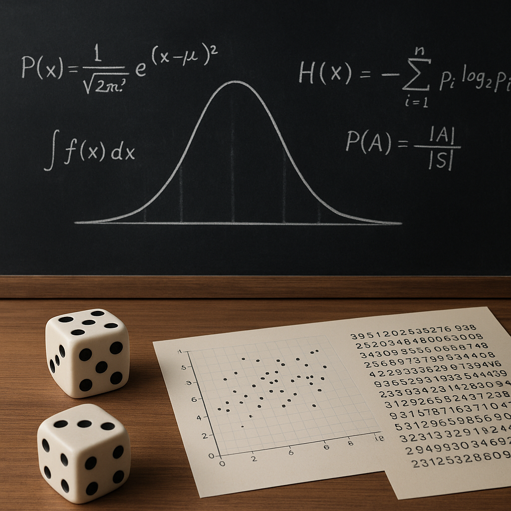
At the heart of any discussion about chance lies the mathematical definition of probability. Informally, probability measures the likelihood of an event occurring, but formalizing this intuitive notion requires a rigorous framework. In this section we explore the building blocks that support modern probability theory.
Probability Spaces
A probability space is defined by a triple (Ω, F, P), where:
- Ω (the sample space) represents all possible outcomes of an experiment.
- F (the σ-algebra) is a collection of subsets of Ω, known as events, closed under complementation and countable unions.
- P (the probability measure) assigns a number between 0 and 1 to each event in F, satisfying axioms of non-negativity, normalization, and countable additivity.
This rigorous setup ensures that probabilities can be manipulated with mathematical precision. The concept of an event’s probability being zero does not necessarily imply impossibility; it merely indicates that the event occurs with negligible frequency in an infinite sequence of trials.
Key Axioms and Properties
Several fundamental properties emerge directly from the axioms:
- Expectation (or expected value) quantifies the long-run average of a random variable: E[X] = Σ x·P(X=x).
- Variance measures dispersion around the expectation: Var(X) = E[(X–E[X])²].
- Independence between two events A and B implies P(A ∩ B) = P(A)·P(B).
Understanding these properties allows for the development of more complex models, including conditional probabilities and transformations of random variables.
Classical Distributions and Their Applications
Probability distributions describe how random variables take on values and form the backbone of statistical modeling. They enable practitioners to capture real-world phenomena—from measurement errors to population dynamics—within a mathematical structure.
Discrete vs. Continuous Distributions
Discrete distributions assign probabilities to countable outcomes, while continuous distributions involve a density function f(x) such that P(a ≤ X ≤ b) = ∫bₐ f(x) dx. Common examples include:
- Binomial Distribution: Models the number of successes in n independent Bernoulli trials.
- Poisson Distribution: Describes the count of rare events in a fixed interval.
- Normal Distribution: Characterized by its bell curve, central to the distribution of errors and natural phenomena.
- Exponential Distribution: Governs waiting times between independent events in a Poisson process.
Each distribution comes with parameters controlling its shape and spread. Statistical inference relies on estimating these parameters from data.
Moments and Characteristic Functions
Moments, such as mean and variance, summarize key features of a distribution. Higher-order moments capture skewness and kurtosis, offering deeper insight into tail behavior. Alternatively, characteristic functions φ(t) = E[eitX] provide a powerful tool for analyzing sums of independent random variables and proving convergence theorems.
Statistical Inference and Estimation
Observational data rarely reveals underlying parameters directly. Statistical inference bridges this gap by using sample data to draw conclusions about populations. Two primary schools of inference—frequentist and Bayesian—offer distinct perspectives on uncertainty and decision-making.
Frequentist Methods
Frequentist inference treats parameters as fixed but unknown, focusing on constructing estimators with desirable properties. Key concepts include:
- Estimator Bias: Difference between expected estimator value and true parameter.
- Confidence Intervals: Ranges that, in repeated experiments, capture the true parameter with a specified probability.
- Hypothesis Testing: Framework for deciding between competing claims using test statistics and p-values.
Maximum Likelihood Estimation (MLE) is a central technique, selecting parameter values that maximize the likelihood of observed data. MLEs often attain asymptotic efficiency under regularity conditions.
Bayesian Framework
In the Bayesian paradigm, parameters are treated as random variables with prior distributions. By applying Bayes’ theorem, posterior distributions combine prior beliefs with evidence from data:
posterior ∝ likelihood · prior
- Prior Distribution: Encodes initial beliefs about parameters before observing data.
- Posterior Distribution: Updated beliefs after incorporating data.
- Bayes Factor: Quantifies evidence for one hypothesis relative to another.
This approach yields full probability distributions over parameters, facilitating direct probability statements and predictive modeling.
Advanced Topics in Randomness
Beyond foundational distributions and classical inference lie sophisticated techniques that leverage computational power and deeper theoretical insights. Here we touch on a few pivotal areas that drive modern research.
Stochastic Processes
A stochastic process is a collection of random variables indexed by time or space, modeling evolving systems under uncertainty. Examples include:
- Markov Chains: Future state depends only on the present state (the Markov property).
- Brownian Motion: Continuous-time process with independent Gaussian increments.
- Poisson Processes: Count of events in disjoint intervals follows independent Poisson distributions.
Applications span queueing theory, financial modeling, and epidemiology, where understanding temporal correlations is crucial.
Monte Carlo Methods
Monte Carlo algorithms employ random sampling to approximate complex integrals and distributions. They are indispensable when analytical solutions are intractable. Key strategies include:
- Rejection Sampling: Generates samples from a target distribution by accepting or rejecting proposals.
- Markov Chain Monte Carlo (MCMC): Constructs a Markov chain whose stationary distribution matches the target.
- Importance Sampling: Weights samples to reduce variance in integral estimates.
Monte Carlo methods underpin simulations in physics, quantitative finance, and machine learning, especially when dealing with high-dimensional spaces.
Randomized Algorithms
Randomness can enhance algorithmic performance and simplicity. Randomized algorithms use random bits to achieve expected runtimes or approximation guarantees. Notable examples include:
- QuickSort: Employs random pivot selection to achieve average-case time O(n log n).
- Las Vegas and Monte Carlo Algorithms: Trade off runtime for guaranteed accuracy or vice versa.
- Hashing and Bloom Filters: Utilize random hash functions for efficient data retrieval with probabilistic error bounds.
By embracing stochastic elements, these algorithms often outperform deterministic counterparts in real-world scenarios.
Emerging Directions
Research continues to push the boundaries, exploring topics such as deep probabilistic programming, uncertainty quantification in artificial intelligence, and the interplay between information theory and randomness. Novel algorithms and theoretical breakthroughs promise to broaden our understanding of chance, enabling more robust decision-making under uncertainty.